RSRP Prediction이 중요한 이유
이제 Downlink Bitrate를 예측했으니, 다음으로 RSRP를 예측할 차례이다.
RSRP Prediction이 중요한 이유는, RSRP 역시 5G 네트워크의 품질 유지와 자원 관리의 핵심 지표이기 때문이다.
1. Handover 안정성 확보
RSRP는 UE가 현재 Cell의 신호 세기를 판단할 때 사용하는 핵심 지표(KPI)이다.
만약 RSRP가 급격히 낮아지면, 연결이 끊어지기 전에 인접 셀로 전환해야 하는데, 정확한 RSRP 예측이 가능하면 이동 중인 사용자의 Proactive Handover를 수행할 수 있다. 이는 곧 신호 약화로 인한 Call Drop이나 패킷 손실을 미리 방지할 수 있다는 뜻이다.
2. Cell 부하 및 자원 최적화
네트워크가 혼잡할 때는 Cell 간 Load Balancing이 필요하다.
RSRP 예측을 통해 각 지역, 시간대별 신호 강도 변화를 미리 파악한다면, Cell Reconfiguration이나 스케줄링 우선순위 조정을 선제적으로 수행할 수 있게 된다. 이는 곧 네트워크 용량을 효율적으로 활용할 수 있음을 뜻한다.
3. QoS 및 사용자 경험 향상
실시간 Application은 일정 수준 이상의 RSRP를 필요로 한다.
RSRP를 예측해 네트워크가 QoS 저하를 미리 감지하고 대응한다면 빔포밍 방향 변경이나 Power Control을 통해 안정적인 연결을 유지할 수 있게 된다. 이는 곧 QoE(사용자 만족도) 향상으로 이어진다.
Feature Selection
마찬가지로 데이터셋은
"Beyond Throughput, The Next Generation: A 5G Dataset with Channel and Context Metrics" 논문을 활용하였다.

앞서, Traffic Prediction에서는 다양한 선행 연구들이 있어서, 이들의 Feature Selection을 그대로 따랐는데,
RSRP에서는 직접 가장 연관성이 높은 Feature들을 찾고, 이들을 Training에 활용해보고자 한다.
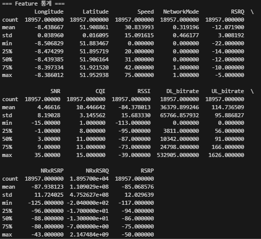
1. 데이터 전처리
우선, 데이터를 확인하고 전처리를 수행한다. (결측치 확인, 통계 확인)
# 데이터 탐색 및 전처리
print("=== 데이터 기본 정보 ===")
print(df.info())
print("\n=== 결측치 확인 ===")
print(df.isnull().sum())
print("\n=== RSRP 통계 ===")
print(df['RSRP'].describe())
이후, 모든 Feature들 중에 사용 가능한 데이터를 추리고, 이들을 Numeric한 수치들로 변경한다.
이 과정에서 PINGAVG와 같이 결측치가 너무 많은 데이터들은 제외한 후, NaN 값을 제거하였다.
이중, 중요한 정보를 담고 있는 NetworkMode는 각각 정수형으로 인코딩을 진행하였다.
# 결측치 처리 및 데이터 준비
df_clean = df[available_features + [target]].copy()

# 데이터 타입 확인
print("=== 데이터 타입 확인 ===")
print(df_clean.dtypes)

# NetworkMode 인코딩 (범주형 변수를 숫자로)
if 'NetworkMode' in df_clean.columns:
    print("\n=== NetworkMode 인코딩 ===")
    print(f"고유값: {df_clean['NetworkMode'].unique()}")
    print(f"각 값의 개수:")
    print(df_clean['NetworkMode'].value_counts())

    # 매핑: 5G=0, LTE=1, 나머지=2
    network_mapping = {
        '5G': 0,
        'LTE': 1,
        'UMTS': 2,
        'HSPA+': 2,
        'HSUPA': 2,
        'HSDPA': 2,
        'HSPA': 2,
    }

    df_clean['NetworkMode'] = df_clean['NetworkMode'].map(network_mapping)
    print("\n인코딩 완료:")
    print("  5G → 0")
    print("  LTE → 1")
    print("  나머지 → 2")
    print(f"\n인코딩 후 값 분포:")
    print(df_clean['NetworkMode'].value_counts().sort_index())

# object 타입 컬럼을 숫자형으로 변환 (숫자가 아닌 값은 NaN으로)
print("\n=== 숫자형 변환 중... ===")
for col in df_clean.columns:
    if df_clean[col].dtype == 'object':
        # 변환 전 샘플 확인
        print(f"  {col}: object -> numeric")
        print(f"    샘플 값: {df_clean[col].unique()[:5]}")
        df_clean[col] = pd.to_numeric(df_clean[col], errors='coerce')
        # 변환 후 NaN 개수 확인
        nan_count = df_clean[col].isna().sum()
        nan_pct = (nan_count / len(df_clean)) * 100
        print(f"    NaN 생성: {nan_count} ({nan_pct:.1f}%)")

# 결측치가 너무 많은 컬럼 제거 (80% 이상이 NaN인 경우)
print("\n=== 결측치가 많은 컬럼 제거 ===")
cols_to_drop = []
for col in df_clean.columns:
    if col == target:
        continue
    nan_pct = (df_clean[col].isna().sum() / len(df_clean)) * 100
    if nan_pct > 80:
        cols_to_drop.append(col)
        print(f"  제거: {col} (NaN {nan_pct:.1f}%)")

if cols_to_drop:
    df_clean = df_clean.drop(columns=cols_to_drop)
    available_features = [f for f in available_features if f not in cols_to_drop]
    print(f"\n남은 Feature 수: {len(available_features)}")

# 결측치 제거 (행 단위)
print(f"\n결측치 제거 전: {len(df_clean)}")
print(f"각 컬럼별 결측치 수:")
print(df_clean.isna().sum())

df_clean = df_clean.dropna()
print(f"\n결측치 제거 후: {len(df_clean)}")

if len(df_clean) < 100:
    print("\n 경고: 데이터가 너무 적습니다!")
    print("   원본 데이터의 값들을 확인해보세요.")
else:
    # 무한대 값 제거
    df_clean = df_clean.replace([np.inf, -np.inf], np.nan).dropna()
    print(f"무한대 값 제거 후: {len(df_clean)}")

    # 변환 후 데이터 타입 확인
    print("\n=== 변환 후 데이터 타입 ===")
    print(df_clean.dtypes)

    # 기본 통계
    print("\n=== Feature 통계 ===")
    print(df_clean.describe())

2. 상관관계 분석 (Correlation Analysis)
# RSRP와 각 feature 간의 상관계수 계산
# 숫자형 컬럼만 사용
numeric_features = [f for f in available_features if np.issubdtype(df_clean[f].dtype, np.number)]
print(f"숫자형 Feature 수: {len(numeric_features)}/{len(available_features)}")
print(f"숫자형 Features: {numeric_features}\n")

correlations = {}
for feature in numeric_features:
    try:
        # 상수 컬럼(모든 값이 같은 경우) 체크
        if df_clean[feature].nunique() > 1:
            corr, p_value = pearsonr(df_clean[feature], df_clean[target])
            correlations[feature] = {
                'correlation': corr,
                'abs_correlation': abs(corr),
                'p_value': p_value
            }
        else:
            print(f"  경고: {feature}는 상수 컬럼입니다. 건너뜁니다.")
    except Exception as e:
        print(f"  오류: {feature} 처리 중 에러 발생 - {e}")

# DataFrame으로 변환 및 정렬
corr_df = pd.DataFrame(correlations).T
corr_df = corr_df.sort_values('abs_correlation', ascending=False)

print("\n=== RSRP와의 상관관계 (절댓값 기준 정렬) ===")
print(corr_df.to_string())

# 시각화
fig, ax = plt.subplots(figsize=(10, 8))
colors = ['red' if x < 0 else 'blue' for x in corr_df['correlation']]
ax.barh(corr_df.index, corr_df['correlation'], color=colors, alpha=0.7)
ax.set_xlabel('Correlation with RSRP', fontsize=12, fontweight='bold')
ax.set_ylabel('Features', fontsize=12, fontweight='bold')
ax.set_title('RSRP와 각 Feature 간의 상관관계', fontsize=14, fontweight='bold')
ax.axvline(x=0, color='black', linestyle='-', linewidth=0.8)
ax.grid(True, alpha=0.3, axis='x')
plt.tight_layout()
plt.savefig('01_Correlation_Analysis.png', dpi=300, bbox_inches='tight')
plt.show()

# available_features를 numeric_features로 업데이트
available_features = numeric_features

=== RSRP와의 상관관계 (절댓값 기준 정렬) ===
             correlation  abs_correlation       p_value
NRxRSRP         0.796850         0.796850  0.000000e+00
RSSI            0.610701         0.610701  0.000000e+00
SNR             0.438467         0.438467  0.000000e+00
CQI             0.363747         0.363747  0.000000e+00
NetworkMode    -0.326196         0.326196  0.000000e+00
Latitude       -0.308681         0.308681  0.000000e+00
RSRQ            0.307287         0.307287  0.000000e+00
Longitude      -0.290804         0.290804  0.000000e+00
DL_bitrate      0.275834         0.275834  0.000000e+00
Speed          -0.148615         0.148615  4.602887e-94
NRxRSRQ         0.115267         0.115267  4.419324e-57
UL_bitrate      0.115173         0.115173  5.446512e-57
(여기서 p-value는 관찰된 상관관계가 우연히 발생했을 확률을 의미한다.)
NRxRSRP가 가장 높은 상관관계를 보임을 관찰할 수 있다.
이를 토대로 히트맵을 그리면 아래와 같다.
# 상관관계 히트맵
plt.figure(figsize=(14, 12))
correlation_matrix = df_clean.corr()
mask = np.triu(np.ones_like(correlation_matrix, dtype=bool))
sns.heatmap(correlation_matrix, mask=mask, annot=True, fmt='.2f',
            cmap='coolwarm', center=0, square=True, linewidths=1,
            cbar_kws={"shrink": 0.8})
plt.title('Feature 간 상관관계 히트맵', fontsize=14, fontweight='bold', pad=20)
plt.tight_layout()
plt.savefig('02_Correlation_Heatmap.png', dpi=300, bbox_inches='tight')
plt.show()

# 강한 상관관계 (|correlation| > 0.3)
strong_corr = corr_df[corr_df['abs_correlation'] > 0.3]
print(f"\n강한 상관관계를 가진 Feature (|r| > 0.3): {len(strong_corr)}개")
print(strong_corr[['correlation', 'p_value']])

2. Random Forest Feature Importance
Random Forest Feature Importance는 모델이 예측할 때 어떤 feature가 중요한지를 정량적으로 평가하는 지표이다.
Random forest란 여러 개의 Decision Tree로 구성된 앙상블 모델이다.
이때 각 Tree는 split하면서 "어떤 변수로 데이터를 나누면 예측 오차가 가장 줄어드는가"를 학습한다.
여기서 Feature Importance는 모델 전체에서 각 feature가 예측 정확도 향상에 기여한 정도를 의미한다.
# Random Forest로 Feature Importance 계산
X = df_clean[available_features].values
y = df_clean[target].values

# 데이터 스케일링
scaler = MinMaxScaler()
X_scaled = scaler.fit_transform(X)

# Random Forest 학습
print("Random Forest 학습 중...")
rf_model = RandomForestRegressor(
    n_estimators=100,
    max_depth=15,
    min_samples_split=10,
    min_samples_leaf=5,
    random_state=42,
    n_jobs=-1
)
rf_model.fit(X_scaled, y)

# Feature Importance 추출
feature_importance = pd.DataFrame({
    'Feature': available_features,
    'Importance': rf_model.feature_importances_
}).sort_values('Importance', ascending=False)

print("\n=== Random Forest Feature Importance ===")
print(feature_importance.to_string(index=False))
결과는 위와 같다. 역시 NRxRSRP가 압도적으로 높은 중요도를 보인다.
결과를 해석해보자면 아래와 같이 정리할 수 있다.
- NRxRSRP: 가장 강력한 predictor — 거의 모델의 70% 이상 영향
- SNR, RSRQ: 전파 품질(Noise 포함)을 반영하는 2차적 신호 지표
- Latitude/Longitude: 공간적 전파 특성을 설명하는 중요한 feature
- RSSI, CQI, Bitrate: 중복 정보나 간접 영향만 있음
이를 그래프로 표현해보면 아래와 같다.
# Feature Importance 시각화
fig, ax = plt.subplots(figsize=(10, 8))
colors = plt.cm.viridis(np.linspace(0.3, 0.9, len(feature_importance)))
ax.barh(feature_importance['Feature'], feature_importance['Importance'],
        color=colors, alpha=0.8)
ax.set_xlabel('Importance Score', fontsize=12, fontweight='bold')
ax.set_ylabel('Features', fontsize=12, fontweight='bold')
ax.set_title('Random Forest Feature Importance', fontsize=14, fontweight='bold')
ax.grid(True, alpha=0.3, axis='x')

# Importance 값 표시
for i, (feature, importance) in enumerate(zip(feature_importance['Feature'],
                                               feature_importance['Importance'])):
    ax.text(importance, i, f' {importance:.4f}', va='center', fontsize=9)

plt.tight_layout()
plt.savefig('03_Random_Forest_Feature_Importance.png', dpi=300, bbox_inches='tight')
plt.show()

# 중요도 상위 Feature
top_important = feature_importance.head(10)
print(f"\n중요도 상위 10개 Feature:")
print(top_important.to_string(index=False))

3. Foward Selection (순차적 Feature 추가)
Forward Selection은 다음 과정을 반복한다.
- 빈 feature 집합(∅) 에서 시작
- 가능한 feature 중 하나를 추가했을 때 모델 성능이 가장 향상되는 feature를 선택
- 선택된 feature를 고정하고, 남은 feature들 중에서 다시 하나를 더 추가
- 더 이상 성능이 개선되지 않거나, 특정 개수에 도달하면 중단
이를 통해 결과적으로 모델 성능에 가장 많이 기여하는 feature들의 조합을 찾는 방법이다.
# 간단한 LSTM 기반 Forward Selection
from tensorflow.keras.models import Sequential
from tensorflow.keras.layers import LSTM, Dense, Dropout
from sklearn.model_selection import train_test_split

def create_sequences_simple(data, target, seq_len=10):
    """간단한 시퀀스 생성"""
    xs, ys = [], []
    for i in range(len(data) - seq_len):
        xs.append(data[i:i+seq_len])
        ys.append(target[i+seq_len])
    return np.array(xs), np.array(ys)

def evaluate_features(feature_list, seq_len=10):
    """주어진 feature 조합으로 LSTM 모델 평가"""
    X_data = df_clean[feature_list].values
    y_data = df_clean[target].values

    # 스케일링
    scaler_X = MinMaxScaler()
    X_scaled = scaler_X.fit_transform(X_data)

    # 시퀀스 생성
    X_seq, y_seq = create_sequences_simple(X_scaled, y_data, seq_len)

    if len(X_seq) < 100:
        return None

    # Train/Test 분리
    X_train, X_test, y_train, y_test = train_test_split(
        X_seq, y_seq, test_size=0.2, random_state=42
    )

    # 간단한 LSTM 모델
    model = Sequential([
        LSTM(32, activation='tanh', input_shape=(seq_len, len(feature_list))),
        Dropout(0.2),
        Dense(16, activation='relu'),
        Dense(1, activation='linear')
    ])
    model.compile(optimizer='adam', loss='mse')

    # 학습 (빠른 평가를 위해 epochs 적게)
    model.fit(X_train, y_train, epochs=20, batch_size=32,
              validation_split=0.1, verbose=0)

    # 평가
    y_pred = model.predict(X_test, verbose=0).flatten()
    mae = mean_absolute_error(y_test, y_pred)
    rmse = np.sqrt(mean_squared_error(y_test, y_pred))

    return {'MAE': mae, 'RMSE': rmse}

print("Forward Selection 준비 완료!")
# Forward Selection 수행 (상위 중요 feature부터 순차 추가)
# 시간이 오래 걸릴 수 있으므로 상위 10개만 테스트

selected_features = []
remaining_features = feature_importance['Feature'].head(10).tolist()
results = []

print("=== Forward Selection 시작 ===")
print("(각 단계마다 LSTM 모델을 학습하므로 시간이 걸릴 수 있습니다)\n")

for step in range(min(7, len(remaining_features))):  # 최대 7개까지만
    best_mae = float('inf')
    best_feature = None

    for feature in remaining_features:
        test_features = selected_features + [feature]
        print(f"Step {step+1}: Testing {test_features}...")

        result = evaluate_features(test_features)
        if result and result['MAE'] < best_mae:
            best_mae = result['MAE']
            best_feature = feature
            best_rmse = result['RMSE']

    if best_feature:
        selected_features.append(best_feature)
        remaining_features.remove(best_feature)
        results.append({
            'Step': step + 1,
            'Feature_Added': best_feature,
            'Features': selected_features.copy(),
            'MAE': best_mae,
            'RMSE': best_rmse
        })
        print(f"  ✓ 추가된 Feature: {best_feature}")
        print(f"    MAE: {best_mae:.4f}, RMSE: {best_rmse:.4f}\n")

forward_results = pd.DataFrame(results)
print("\n=== Forward Selection 결과 ===")
print(forward_results.to_string(index=False))
이를 통해 출력된 결과는 아래와 같다.


4. LASSO 회귀 (LASSO Regression)
LASSO 회귀는 불필요한 변수의 가중치를 자동으로 0으로 줄이는 회귀 기법이다.
이는 곧 Feature Selection을 자동으로 수행한다고 할 수 있다.

보통 회귀모델은 아래처럼 “오차를 최소화”하려고 학습한다.

LASSO는 여기에 규제항(regularization term)을 하나 더 추가한다.
여기서 βi는 각 특성(feature)의 계수이고, λ는 얼마나 강하게 규제할지 정하는 파라미터이다.
이때 λ가 커질수록, 중요하지 않은 특성의 βi가 0이 되어 자동으로 제외된다.
from sklearn.linear_model import Lasso
from sklearn.preprocessing import MinMaxScaler
import numpy as np
import matplotlib.pyplot as plt

# ====== 1. 데이터 준비 ======
X = df_clean[available_features].values
y = df_clean[target].values

# ====== 2. 스케일링 (LASSO는 스케일 민감함) ======
scaler_X = MinMaxScaler()
X_scaled = scaler_X.fit_transform(X)

# ====== 3. Alpha 변화에 따른 계수 계산 ======
print("=== LASSO Path 계산 중... ===")
alphas = np.logspace(-4, 1, 100)
coefs = []

for alpha in alphas:
    lasso_temp = Lasso(alpha=alpha, max_iter=10000, random_state=42)
    lasso_temp.fit(X_scaled, y)
    coefs.append(lasso_temp.coef_)

coefs = np.array(coefs)

# ====== 4. LASSO Path 시각화 ======
fig, ax = plt.subplots(figsize=(12, 7))

for i, feature in enumerate(available_features):
    ax.plot(alphas, coefs[:, i], label=feature, linewidth=2)

ax.set_xscale('log')
ax.set_xlabel('Alpha (정규화 강도)', fontsize=12, fontweight='bold')
ax.set_ylabel('Coefficient 값', fontsize=12, fontweight='bold')
ax.set_title('LASSO Path: Alpha 값에 따른 계수 변화', fontsize=14, fontweight='bold')
ax.axhline(y=0, color='black', linestyle='--', linewidth=0.5, alpha=0.5)
ax.legend(bbox_to_anchor=(1.05, 1), loc='upper left', fontsize=9)
ax.grid(True, alpha=0.3)
plt.tight_layout()
plt.show()

print("\n💡 해석:")
print(" - Alpha가 커질수록 LASSO의 정규화 강도가 세져서 더 많은 계수가 0으로 수축됩니다.")
print(" - Alpha가 커져도 0이 되지 않는 Feature는 RSRP 예측에 가장 중요한 변수입니다.")
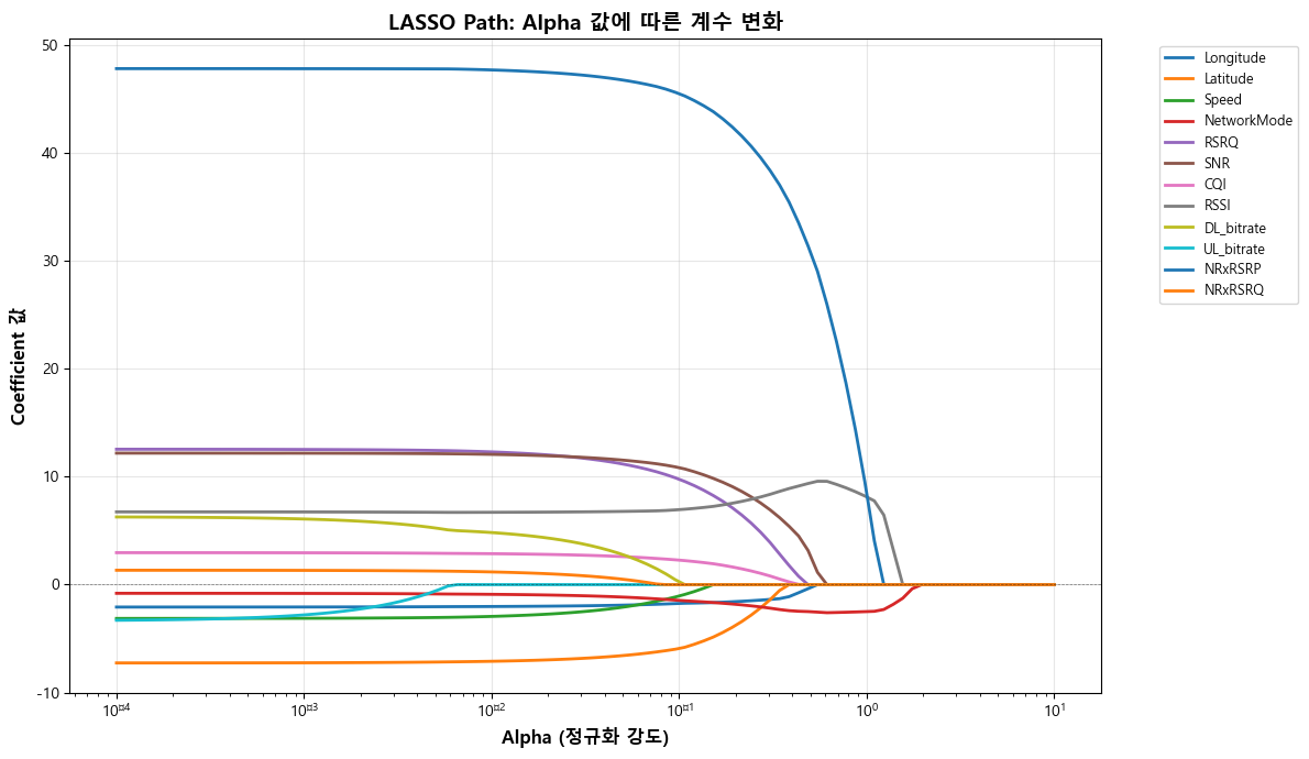
이를 통해 LASSO가 강하게 규제해도 여전히 유의미한 변수들이 뭔지를 확인할 수 있다.
NetworkMode가 정규화가 아무리 강해도 끝까지 남은 변수로, LASSO가 중요한 변수로 판단했음을 알 수 있다.
또한, NRxRSRP의 절대 계수 역시 상당히 큰 것을 보아 실제 영향력 측면에서는 여전히 최상위 변수임을 보인다.
'딥러닝 모델 > LSTM for Traffic Prediction' 카테고리의 다른 글
| UE Trajectory 예측 Task를 위한 LSTM과 LLM의 비교 (0) | 2025.10.29 |
|---|---|
| RSRP 예측 Task에 대한 LSTM과 LLM의 비교 (0) | 2025.10.28 |
| LSTM 학습과 관련된 몇 가지 Technique (0) | 2025.10.27 |
| Downlink Throughput 예측 Task에 대한 LSTM과 LLM의 비교 (0) | 2025.10.27 |
| LSTM 모델로 실제 Downlink Throughput 예측하기 (0) | 2025.10.24 |